
Learning to design a stage costume requires more than producing a visually convincing garment. Students must interpret a performance brief, investigate relevant forms, justify material choices, communicate with collaborators, construct an artefact, and evaluate the relationship between an intention and its physical expression. Instructional achievement therefore concerns several connected forms of judgement and action. A single course score can summarise these activities, but it cannot independently establish which capability changed or whether a student can exercise that capability without assistance. This distinction becomes consequential when comparative course evaluations are used to recommend one instructional approach over another. The educational question concerns what students can do; the evidential question concerns what the available observations can establish.
Design-based learning places the production of an artefact within a process of inquiry, knowledge application, and iterative decision-making. The defining characteristics identified by Gómez Puente and colleagues include the nature of the design task, the learning activities, teacher involvement, assessment, and the social setting [1]. These characteristics are interdependent. A task may permit different solutions while assessment rewards only a narrow form of execution, or students may exercise substantial choice while receiving intensive technical assistance. Consequently, the instructional label does not specify a uniform treatment. Comparisons require attention to what learners decided, what teachers supplied, and which aspects of the resulting work were evaluated. Otherwise, differences in course organisation can be mistaken for differences in students’ independent design competence.
Design thinking provides related accounts of problem interpretation, idea generation, prototyping, feedback, and further development. Razzouk and Shute describe an interaction between analytic and creative activity that is relevant to learning through design [2]. The relationship between design thinking and design-based learning nevertheless requires care: one can describe a way of approaching problems, while the other describes an arrangement of educational activity. A course can employ both without making the terms interchangeable. The Educational Design Ladder similarly places educational development within differentiated levels of engagement, rather than treating exposure to design terminology as sufficient evidence of expertise [3]. For costume education, this directs attention to the decisions embodied in the work and to the level of responsibility actually assumed by the student.
The literature also offers reasons to examine instructional enactment alongside nominal course structure. Henriksen and colleagues discuss design thinking as a means of working through educational problems, connecting creative inquiry with the difficulties encountered in practice [4]. Panke’s synthesis documents variation in educational uses, purposes, and limitations across settings [5]. These accounts support examining how design activity is organised, but they do not establish that every implementation produces the same learning outcome. In particular, successful engagement with an open task and superior performance on a course assessment are related propositions with different evidential requirements. Neither proposition alone demonstrates long-term retention, transfer to a different brief, or improved professional performance.
Quantitative research strengthens the case for taking design-oriented teaching seriously while also making the conditions of comparison more visible. A meta-analysis found a positive association between design-thinking instruction and student learning, with differences associated with outcome and implementation characteristics [6]. In higher education, a study involving multiple assessment perspectives examined problem solving and creativity across a semester [7]. Its attention to students, peers, and facilitators is especially relevant because the assessment perspective forms part of the interpretation. An instructor’s judgement of a completed project, a student’s judgement of personal progress, and a peer’s judgement of collaboration answer different questions. Agreement among them can be useful, but an average across perspectives does not eliminate their distinct meanings.
Studio assessment presents a corresponding problem of representation. Research, communication, production, presentation, and reflection can be expressed through different kinds of evidence, even when they contribute to a common score. A well-constructed object may reveal technical control while providing limited evidence about the reasoning that preceded it. A persuasive presentation may reveal communication without resolving how much of the construction was completed independently. Dawson’s analysis of rubric design makes clear that the term rubric encompasses consequential differences in criteria, levels, descriptions, and use [8]. Reporting a numerical scale is therefore insufficient to establish what a one-point difference means educationally. The interpretation also depends on what was observed, how the judgement was made, and whether the same expectations were applied across groups and occasions.
Feedback further complicates any attempt to separate instruction mechanically from assessment. In studio teaching, comments can contribute to the development of the work that is subsequently graded. Carless and Boud identify students’ capacities to interpret and act on feedback as central to its productive use [9]. Tai and colleagues place the ability to judge the quality of one’s own and others’ work within the purposes of higher education [10]. These perspectives make reflection and critique educationally meaningful, but they also encourage precise outcome descriptions. Improvement in an assessed project can involve better use of feedback, more effective collaboration, increased familiarity with criteria, and stronger technical execution. Published course summaries do not necessarily permit those contributions to be separated.
The distinction between self-perception and demonstrated performance is particularly relevant to creative work. A meta-analysis of creative self-efficacy found that its relationship with creativity depended on the form of assessment, including whether creativity was self-rated or assessed through performance procedures [11]. Confidence in one’s design ability should consequently be interpreted as a potentially relevant psychological attribute rather than a substitute for evidence of design achievement. Likewise, a teacher-rated score should retain its status as a judgement made under specified educational conditions. Treating either type of observation as direct evidence of a broad, context-independent ability obscures the task, the evaluator, and the assistance through which that observation arose.
Motivation provides another substantive reason to avoid reducing design learning to a single instructional contrast. Self-determination theory differentiates the reasons for engaging in an activity and distinguishes autonomous from more controlled forms of regulation [12]. These distinctions are pertinent to costume projects because interest in making, a desire to demonstrate achievement, and concern about failure need not carry identical implications for participation. Large educational syntheses associate different motivational forms with different outcomes and identify psychological need satisfaction and autonomy support as relevant correlates of student motivation [13], [14]. Such findings support examining motivation carefully. They do not allow a motivation coefficient from a particular course to establish that the measured motive caused the assessed achievement.
Research on creativity reinforces the need for specificity. A synthesis of intrinsic motivation and creative products identified a positive relationship, while work on everyday creativity showed that the importance of particular motives differed across creative domains [15], [16]. These findings make it plausible that enjoyment, challenge, expression, recognition, and obligation can have different roles in creative participation. They do not establish that a broad motivation total captures those roles equally well. In a course evaluation, motivation may also be related to earlier competence, familiarity with the task, teacher interaction, or the experience of receiving a favourable assessment. Without appropriate temporal and individual information, these possibilities remain observationally entangled rather than empirically distinguished explanations.
The present investigation addresses a narrower question about the strength of instructional achievement conclusions available from cited work. A difference between groups at the final assessment, a difference between their average changes, and a difference interpreted as an instructional effect are distinct quantities. The first two can sometimes be calculated from group means even when individual records are unavailable. Their uncertainty, however, depends on additional information. In particular, repeated assessments on the same student are related, and that relationship enters the variance of the student’s change. Two groups can therefore have precisely the same published means and standard deviations while yielding different uncertainty estimates for the contrast in improvement.
Adjustment for initial achievement presents a related but distinguishable identification problem. In a common-slope analysis of covariance, the fitted instructional coefficient depends on the within-group association between initial and final scores. Nevertheless, the size of the possible adjustment is constrained by the observed standard deviations and by the difference between the initial group means. A missing covariance therefore need not imply that every adjusted group difference is possible. Establishing the full compatible range can reveal whether covariance uncertainty is consequential for the sign or magnitude of the instructional contrast. This question differs from choosing an assumed correlation and presenting the resulting regression as uniquely determined. It also differs from estimating the causal effect of instruction, which requires assumptions about assignment and potential outcomes beyond the covariance identity. The analysis developed here uses this distinction to retain the adjusted-comparison method while making the information required for its interpretation explicit.
Collaboration introduces a second level of dependence. Students working in teams of three share task decisions and may receive common feedback or respond to the same production difficulty. This does not establish that their final scores are identical, nor that all dependence is attributable to teamwork. It establishes a reason to examine how inference changes when observations within a team are related. The relevant uncertainty cannot be resolved simply by counting students. At the same time, introducing a numerical allowance for team dependence does not recover unreported team identities or estimate an observed intraclass correlation. Its purpose here is conditional: to show the consequences of specified dependence assumptions for conclusions drawn from the available summaries.
A third consideration is whether the score contrast is sensitive to differential evaluation. An additive rating offset provides a direct way to ask how much systematic elevation of one group’s ratings would be needed to alter a stated conclusion. This quantity describes a sensitivity threshold; it is not evidence that any evaluator applied such an offset. It is useful because it is expressed on the same scale as the course assessment and can be compared with the observed contrast. Numerical rounding requires a separate check. Means and standard deviations printed to limited precision represent intervals of possible values, so the apparent exactness of a derived quantity should not exceed the precision of its inputs.
The research question is therefore: which conclusions about comparative instructional achievement remain defensible when the pre–post covariance is unknown, printed summaries are rounded, students work in teams of three, and a differential additive rating offset is allowed? The analysis preserves the reported teaching and assessment context while distinguishing quantities calculable from the summaries from quantities requiring additional assumptions. Its contribution is a set of explicit numerical conditions for interpretation, rather than a claim to have observed a new cohort or identified a causal mechanism. The resulting evidence can support a bounded statement about assessed achievement and its sensitivity. Claims about independent capability, motivational causation, retention, or transfer require observations that the numerical summaries do not provide.
The computational dataset contains group counts, pre-instruction and post-instruction means, standard deviations, and selected model summaries [17]. The students were third-year undergraduates aged 19–23 years, recruited purposively from Kazan Federal University and Kazan State Institute of Culture in the Republic of Tatarstan, Russia. Group division is described as random, but the allocation sequence, concealment procedure, and relationship between institutional membership and instructional assignment are not documented sufficiently to verify randomization. Accordingly, the estimand is an observed contrast between instructional groups, with uncertainty conditional on explicit statistical assumptions. Neither a new student cohort nor additional classroom experiments were conducted for the present calculations.
The teaching sequence comprised stage-costume sketching, model development, material selection, manufacture, and presentation. Both instructional groups completed comparable assignments in teams of three. In design-based learning, students made design decisions with teacher assistance, received feedback, and selected how to present their work. In teacher-directed instruction, the teacher explained and guided the construction sequence and supplied a presentation plan. The documented construction phase comprised eight weeks with three 90-minute lessons weekly, equivalent to 36 contact hours; the presentation phase comprised four weeks on the same timetable, equivalent to 18 hours. These descriptions establish 54 hours for those two phases, without establishing the duration of all preparatory activity. The comparison therefore concerns two ways of organizing collaborative design work, rather than the presence versus absence of practical costume production.
Assessment used the control and final diagnostic sheets (CFDS), comprising 30 items: five sheets with five items each for research, communication, product creation, presentation, and reflection, together with five items assessing the completed art project. Table 1 provides communication criteria and observational indicators, including listening, discussion, and collaboration. This is evidence about assessed behaviors, not a complete scoring specification. The report gives internal consistency of 0.90, average variance extracted of 0.51, and composite reliability of 0.77 for CFDS. These quantities do not establish agreement between assessors or invariance of scoring across instructional groups. Such distinctions are necessary when interpreting ratings of complex performance [18], [19]. Response anchors, item weights, assessor-level scores, assessor independence, and masking to instructional membership were unavailable and are not reconstructed.
The Table 1 labels establish the primary allocation of 102 students to teacher-directed instruction and 105 to design-based learning. Because the used abstract reverses those counts, a separate calculation exchanges the sample sizes while retaining each instructional group’s reported means and standard deviations. This check isolates the consequence of the count discrepancy; it does not determine which participant-level allocation was used.
| Instruction | \(n\) | Pre mean | Pre SD | Post mean | Post SD |
|---|---|---|---|---|---|
| Teacher-directed | 102 | 2.44 | 0.55 | 3.71 | 0.40 |
| Design-based | 105 | 2.41 | 0.55 | 4.19 | 0.42 |
The input contrast combines a small initial mean difference with a larger final difference. Both groups have identical displayed initial dispersion, whereas final dispersion is slightly greater under design-based learning. This information identifies unadjusted mean differences and several variance bounds, but does not identify paired changes, conditional regressions, or team covariance uniquely. Table 3 supplies an instructional ANCOVA with an error degree of freedom of 204; that denominator is used when checking its effect-size arithmetic. Tables 5 and 6 provide gender summaries, and Table 7 provides a multivariable regression display. Their retention as documentary evidence does not make their underlying analyses recoverable from the available margins.
All displayed means and standard deviations are treated first as the numerical inputs shown, then as rounded quantities within \(\pm0.005\). Counts are integers and are not subjected to rounding intervals. The resulting calculations distinguish exact arithmetic on displayed numbers from enclosures that allow numerical precision to vary. Reported \(p\) values, standard errors, and adjusted means are compared for compatibility rather than used to manufacture missing observations. In particular, no domain-level values are estimated from the coordinates in published plots, and no item-level data are simulated. This treatment makes the information available for inference explicit, consistent with recommendations to disclose measurement and analytic decisions [20].
Let \(C\) denote teacher-directed instruction, \(D\) design-based learning, \(X\) the initial CFDS score, and \(Y\) the final score. The final mean contrast is positive when the design-based group has a higher rating. Under independent sampling of students, its estimated standard error and Welch interval are
where \(\nu\) is the Welch–Satterthwaite degree of freedom. This interval describes sampling uncertainty under independence; it does not adjust instructional selection, common assessors, or shared team work. A standardized contrast complements the score-unit estimate, following the distinction between effect magnitude and statistical significance [21]:
The exact gamma-function correction avoids an unnecessary approximation to the small-sample adjustment [22]. The denominator is the pooled final standard deviation, so \(g\) measures separation relative to final dispersion. It is not a standardized within-person improvement or a measure of design proficiency outside CFDS. The raw contrast remains primary because its relationship to an additive rating offset is directly interpretable. Initial-score contrasts are calculated with the same independent-samples logic as an arithmetic check, without using their significance as a criterion for accepting comparability. A small observed initial difference cannot demonstrate balance on unmeasured design experience, prior instruction, assessor expectations, or institutional conditions. The analysis therefore reports initial similarity as a property of the available CFDS summary rather than as validation of instructional assignment. No educationally important difference is imposed because an independently established CFDS threshold was unavailable.
The mean change contrast is identified by four group means even when paired records are unavailable:
Its uncertainty depends on the association between initial and final scores. Consequently, reporting a change-score test requires more information than subtracting group means, an issue central to inference for pretest–posttest designs [23]. For group \(j\in\{C,D\}\), let \(\rho_j\) denote the unreported within-student correlation. Then
The complete correlation domain \([-1,1]^2\) is examined, with \(\rho_C\) and \(\rho_D\) allowed to differ. Nonnegative correlations are additionally displayed as an interpretable subset, without treating them as observed. Variance increases monotonically as either correlation decreases, placing the largest variance at \(\rho_C=\rho_D=-1\). These limits are algebraically admissible given the supplied moments; unspecified score support or item constraints could narrow them. Conditional Welch intervals use the correlation-dependent group variances. A conservative enclosure instead applies the larger critical value associated with \(\min(n_C-1,n_D-1)\) to the largest variance, avoiding a claim that maximizing standard error alone exactly maximizes a Welch endpoint.
Initial-score adjustment and change-score analysis answer different questions and can behave differently when instructional membership is not demonstrably randomized [24], [25]. The retained ANCOVA has an intercept, group indicator, and common linear slope \(b\) for \(X\). With \(S_{XX}=\sum\limits_j(n_j-1)s_{Xj}^{2}\), \(S_{YY}=\sum\limits_j(n_j-1)s_{Yj}^{2}\), and within-group cross-product \(S_{XY}\), its adjusted group coefficient satisfies
The bound follows from applying the covariance inequality separately within each group and summing the allowable cross-products. For the displayed values, \(B=0.74572062\) and \(\widehat\tau(b)=0.48+0.03b\). The resulting coefficient interval is therefore determined by the small initial imbalance and the maximum slope permitted by the observed dispersions. It is a set of compatible coefficients, not a confidence interval, and does not assert that a common linear relationship is substantively correct.
Under the additional assumptions of independent observations and normally distributed, homoscedastic linear-model errors, a conditional standard error is available for every admissible slope:
Taking the union of the associated \(t_{N-3}\) intervals produces a conditional uncertainty envelope over the unidentified covariance. This envelope preserves uncertainty about pairing while keeping the regression assumptions visible. For reproducibility, write \(A=1/n_C+1/n_D+(\bar X_D-\bar X_C)^2/S_{XX}\) and \(k=t_{0.975,N-3}\sqrt{A/(N-3)}\). When the optimizing slopes lie within the feasible interval, as they do here, the envelope is
This expression includes the movement of the coefficient and its conditional standard error simultaneously. Evaluating only the largest allowable slope would miss the interior slope at which an interval endpoint is most extreme. The envelope is not a replacement for a regression with observed covariances, heteroscedasticity checks, and recorded clusters. The instructional effect-size entry in published Table 3 is checked using partial eta squared, \(F/(F+204)\), because its numerator degree of freedom equals one. Neither the reported slope-homogeneity test nor rounded adjusted means supplies the missing group covariances.
A dependence calculation represents the documented teams of three by a common nonnegative within-team correlation \(\rho_T\). With equal team size, the variance inflation is
This familiar design-effect expression describes exchangeable within-team dependence [26]; it is used as a sensitivity calculation, not evidence that instruction was assigned by team. The displayed counts permit 34 and 35 intact teams, yielding an illustrative critical value with 67 degrees of freedom. Neither team membership nor an intraclass correlation was reported. The calculation therefore varies \(\rho_T\) from zero to one and does not imply that 69 independently sampled teams actually existed. Institution-level dependence, teacher effects, unequal team sizes, and cross-team interaction require records unavailable here. The equal-team calculation also assumes the same intraclass correlation in both instructional groups. In the extreme case of perfectly correlated ratings within each team, the design effect reaches three. This upper endpoint demonstrates the largest inflation under the stated three-person exchangeable model, rather than a universal limit on dependence. Clustering by a teacher or institution could involve many more students and would not be bounded by that endpoint.
Assessment sensitivity is represented by a differential additive offset \(\delta_B\) on the design-based group’s final scores. Its offset-adjusted contrast is
The offset that makes the point contrast zero differs from the smaller offset that makes a lower interval endpoint zero. Reporting both prevents these two evidentiary questions from being conflated. A constant group offset changes means without changing within-group dispersion; heterogeneous assessor effects would require a richer model. This calculation quantifies sensitivity to one explicit measurement departure. It does not estimate assessor bias or correct selection into instruction. Sensitivity to omitted-variable confounding would require a distinct parameterization and additional covariate information [27].
Finally, rounded-value intervals are propagated through contrasts, variance limits, and slope bounds using endpoint calculations or conservative interval enclosures. The eight continuous inputs comprise four means and four standard deviations. Each is allowed to vary independently over its rounding interval because additional constraints from the scoring procedure are unknown. For functions with established endpoint extrema, all relevant corners are evaluated; otherwise, the report identifies the enclosure as conservative. This distinction prevents numerical precision checks from implying reconstruction of undisclosed digits. Correlation uncertainty and rounding uncertainty are combined when assessing the change contrast, so the most favorable pairing is never silently paired with the least favorable displayed mean. The count-reversal calculation is repeated independently. Gender claims are restricted to what published Tables 5 and 6 support. The participant description totals 56 male and 151 female students, whereas Table 6 lists 51 and 156. Table 5 places 33.48 in its error degrees-of-freedom position, which cannot be interpreted as the integer residual degree of freedom of the stated ordinary ANCOVA. These discrepancies are recorded explicitly; neither the sample split nor a corrected inferential result is guessed. A nonsignificant or threshold-level result is not treated as evidence of equivalence [28]. Published Table 7 is retained as a description of a reported association analysis; its designation as logistic regression cannot be reconciled from the supplied standardized coefficients and \(t\) statistics without an outcome definition and model specification. No motivation coefficients are refitted, and no causal mediation is inferred. The accompanying executable analysis records every numerical input, formula, and sensitivity parameter needed to reproduce the aggregate calculations.
The instructional groups differ by 0.480 points at posttest. The standard error calculated from the two sample sizes and within-group standard deviations is 0.057, giving a Welch interval from 0.368 to 0.592 points. The pooled posttest standard deviation is 0.410, and the bias-corrected standardized difference is 1.166. These calculations establish a pronounced separation relative to the dispersion of the recorded ratings. They do not establish the practical value of a point on the diagnostic instrument, because complete scoring anchors and an independently justified educational threshold are unavailable. A standardized contrast describes the relationship between a mean difference and sample variability; it is not a measure of professional competence or a guarantee that a comparable instructional change would reproduce the same outcome elsewhere.
Because the complete CFDS scoring key is unavailable, a difference of 0.480 points cannot be converted reliably into a percentage of the attainable score. The analysis therefore retains the rating unit and avoids assigning unverified proficiency categories to either instructional group.
The pretest difference, expressed in the same direction, is \(-0.030\) points. The associated group means are close, but closeness on one measured outcome cannot establish comparability on prior costume-making experience, instructor expectations, access to materials, or other determinants of assessed performance. Moreover, a pretest significance test addresses a sampling calculation under specified assumptions; it does not verify the allocation process. Statistical significance also supplies neither a measure of educational importance nor a probability that a substantive explanation is correct [29]. The aggregate records consequently support an explicit adjustment analysis without allowing a broader claim that all relevant initial conditions were equal. The detectable separation in this fixed sample does not establish adequate precision for subgroup or transfer questions; sample adequacy depends on the particular inferential objective [30].
| Quantity | Estimate | Interval or admissible range |
|---|---|---|
| Posttest difference, points | 0.480 | [0.368, 0.592] |
| Hedges’ \(g\) | 1.166 | — |
| Difference in mean changes, points | 0.510 | Correlation-dependent |
| ANCOVA group coefficient, points | Unidentified | [0.458, 0.502] |
| ANCOVA confidence-set envelope, points | — | [0.365, 0.595] |
| Posttest difference after rounding, points | — | [0.470, 0.490] |
| Posttest confidence limits assume independent students. The ANCOVA coefficient range is an algebraic bound; its confidence-set envelope additionally assumes independent, homoskedastic errors. Rounding limits describe numerical admissibility, not sampling uncertainty. All quantities are calculated from the aggregate inputs credited in Section II. | ||
The quantities in Table 2 answer different questions. The posttest interval describes uncertainty under a sampling model, whereas the adjusted-coefficient range describes ambiguity created by missing covariance information. Combining them into a single undifferentiated measure would obscure the distinction between sampling variation and incomplete numerical specification. The standardized difference is presented alongside the raw contrast to retain the original rating unit. Reporting both quantities also prevents the small within-group posttest dispersion from becoming the sole basis for judging educational importance.
The admissible common slope spans \(-0.746\) to \(0.746\), yet the corresponding group coefficient spans only 0.458 to 0.502 points. The total width of the latter range is 0.045 points. Its narrowness follows directly from multiplying the admissible slope by the small pretest mean difference. Adjustment can vary markedly at the student level without greatly changing the difference between group means when those pretest means are similar. This is the substantive algebraic reason that the aggregate instructional contrast remains positive across the covariance choices considered here.
The result does not require selecting a preferred within-person correlation. Both positive and negative group-specific correlations are admitted, subject to compatibility with the printed standard deviations. Nor does the calculation recover which covariance actually occurred. The endpoints describe possible fitted coefficients under the common-slope model. They should not be read as confidence limits, as a probability distribution over coefficients, or as uncertainty about every possible model of learning. An interaction between instructional group and pretest achievement would define a different estimand whose empirical adequacy cannot be assessed from these margins alone.
The relationship displayed in Figure 1 separates the coefficient range from conditional sampling uncertainty. The fitted group difference changes linearly with the admissible slope, whereas the width of its conventional interval depends on residual variation. The union of those intervals extends from 0.365 to 0.595 points. This envelope is wider than the coefficient range because it combines covariance ambiguity with a particular error model. It remains an approximate confidence set conditional on the supplied summaries and the model assumptions; it does not account for instructor effects, unmeasured selection, or systematic differences in scoring. Such qualifications are intrinsic to confidence-interval interpretation, because numerical coverage under an assumed model does not include every potential source of bias [31].
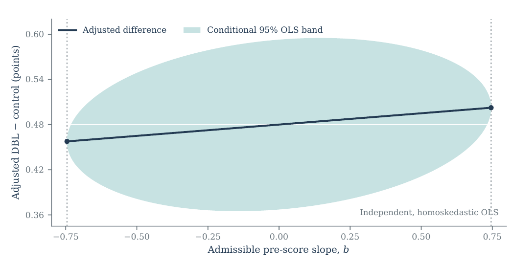
The adjusted group means printed in the numerical materials differ by 0.490 points, which falls inside the calculated coefficient range. This agreement establishes compatibility with the aggregate moments, rather than reproduction of the fitted analysis. The reported group \(F\) statistic of 73.17, together with residual degrees of freedom of 204, gives partial eta squared of 0.264. Agreement with the displayed value of 0.26 is a successful arithmetic check. It supplies no missing covariance matrix and does not validate every entry in the accompanying statistical tables. A reproducible assessment should identify both successful and unsuccessful checks with equal specificity.
Allowing each posttest mean to vary within its two-decimal rounding interval moves the instructional contrast only between 0.470 and 0.490 points. The direction of the difference is therefore insensitive to that numerical precision. The endpoints are not alternative observations; they are the limiting values permitted by the printed numbers under ordinary nearest-value rounding. This distinction matters because additional decimal places in the computational files express arithmetic precision, while the manuscript retains reporting precision appropriate to its inputs.
Jointly allowing rounding of the means and standard deviations expands the adjusted-coefficient limits to 0.440–0.520 points. The corresponding conventional confidence-set envelope becomes 0.352–0.608 points. The coefficient-range width consequently increases from approximately 0.045 to 0.081 points, because rounding alters both the pretest mean difference and the admissible adjustment slope. This interaction explains why examining the posttest rounding interval alone understates numerical uncertainty in the adjusted contrast. Nevertheless, the expanded coefficient set remains positive. The confidence-set envelope is a separate, wider statement: it also includes residual sampling variation under the common-slope error model. Neither expansion repairs uncertainty about allocation or scoring, and neither assigns probability to the values permitted by rounding. Their contribution is to show how the conclusion changes when printed precision and missing pairing are considered together.
The mean increases are 1.270 points for teacher-directed instruction and 1.780 points for design-based learning. Their difference is 0.510 points, or between 0.490 and 0.530 points when all four means are allowed to vary within their rounding intervals. Subtracting the pretest means therefore increases the posttest contrast by 0.030 points. That arithmetic does not establish that each learner improved. A positive change in a group average is compatible with heterogeneous individual trajectories, including no change or declining scores for some participants. Individual improvement rates and the association between initial performance and subsequent change require linked records.
The uncertainty of the difference in changes is substantially less stable than its point estimate. With both within-group correlations equal to \(-1\), the conditional Welch interval is 0.247–0.773 points. At zero correlation it is 0.322–0.698, and at a correlation of one it narrows to 0.471–0.549. The standard errors at the extreme corners differ by a factor of approximately 6.83. Thus, the same marginal summaries support a stable average contrast together with a wide range of possible precision statements about change.
The two-dimensional calculation in Figure 2 admits different pre–post correlations in the two instructional groups. Its purpose is to display how pairing information changes uncertainty without changing the observed marginal means. The largest change variance occurs when both correlations are negative at their admissible extremes; the smallest occurs when both are positive at their extremes. The full square of admissible correlations avoids assuming that the two instructional approaches produced the same relationship between initial and final achievement.
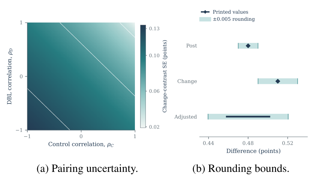
The rounding comparison in the same display is deliberately separate from the correlation surface. Numerical precision perturbs the means and standard deviations within narrow intervals, whereas missing pairing alters the relationship between repeated measurements. Neither calculation estimates a distribution of possible correlations or rounding errors. Treating the illustrated values as equally probable would add assumptions unsupported by the available materials. The findings instead identify which conclusions follow from the margins alone and which require information that the margins do not contain. Integer-score checks such as GRIM require known score granularity [32]. The incomplete scoring specification does not justify applying those restrictions to these rubric aggregates; the present calculations test rounding intervals and stated algebraic identities only.
The documented use of three-person teams introduces a plausible source of dependence between student ratings. Shared materials, discussion, and joint production can align outcomes within a team even when the final assessment is recorded for each student. Dividing the teaching-group counts by three gives 34 and 35 potential complete teams. These are inferred counts conditional on intact membership; the numerical materials do not provide an observed team roster. They support an illustrative dependence calculation, not an empirically fitted multilevel model.
Under an equal-size exchangeable model, increasing the intraclass correlation from zero to one multiplies the variance by a factor from one to three. Using the same illustrative 67-degree-of-freedom convention throughout this calculation gives a posttest interval of 0.366–0.594 points at zero intraclass correlation and 0.283–0.677 points at one. The positive lower limit at maximal dependence within teams shows that the observed separation does not rely solely on treating three closely collaborating students as fully independent. It does not establish robustness to dependence at larger organizational levels. Two institutions, a small number of classrooms, or common instructors could generate covariance patterns that are not represented by a three-person design effect.
Systematic assessment differences address another issue entirely. If design-based learning ratings exceed otherwise comparable ratings by an additive amount \(\delta_B\), the displaced instructional contrast is \(0.480-\delta_B\). A displacement of 0.480 points removes the point difference. Under the independent-student calculation, a displacement of approximately 0.368 points moves the lower confidence limit to zero. Under maximal team dependence with the stated degrees of freedom, that threshold is approximately 0.283 points. These thresholds quantify the size of a specified offset required to change a conclusion; they do not estimate whether such an offset occurred.
Allowing two-decimal rounding together with maximal dependence within three-person teams reduces the lower interval endpoint to approximately 0.271 points. This is also the additive offset that removes the positive lower limit under those combined assumptions; it remains a conditional threshold, not an estimated assessment difference.
The joint display in Figure 3 makes the distinction visible. Increasing team dependence widens the interval around the same displaced estimate. Increasing the additive offset shifts the interval itself. The zero contour therefore marks combinations of assumptions under which a positive lower limit ceases to hold. No location on the plot is assigned a probability, and the observed study cannot be placed at a unique coordinate because neither the intraclass correlation nor the offset is known.
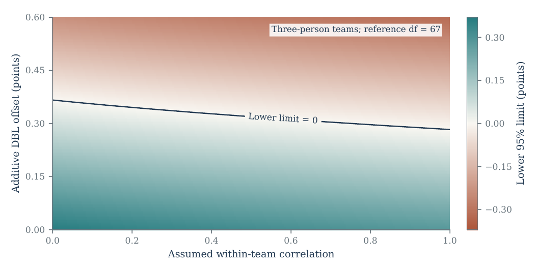
A teacher who both supports design work and evaluates it may observe authentic learning that a detached assessment misses, but may also apply expectations differently across instructional conditions. The aggregate evidence cannot separate these explanations. The sensitivity calculation preserves that ambiguity while making its numerical consequences explicit. It also prevents an attractive but invalid inference: that a large standardized difference must be resistant to systematic scoring differences. Sampling uncertainty can be small even when the measurement process contains an unestimated group-specific shift.
The reporting checks distinguish limited precision from algebraic incompatibility. Computational checking of reported statistical relationships can identify discrepancies while leaving their explanation unresolved [33]. Weighting the instructional means by their sample sizes gives an overall posttest mean of 3.9535. Weighting the gender means printed in the descriptive gender table gives 3.9571. Their difference of approximately 0.0036 points is compatible with two-decimal rounding. This comparison therefore supplies no basis for declaring those overall means inconsistent. In contrast, the participant description totals 56 men and 151 women, while the gender table lists 51 and 156. Rounding cannot reconcile integer counts, and the available materials do not establish which classification is correct.
Reversing the instructional sample counts provides a numerical check on the conflicting allocation totals. The posttest interval then becomes 0.3675–0.5925 points and Hedges’ \(g\) becomes 1.167, compared with 1.166 under the tabulated allocation. The limited movement follows from the similar group sizes and posttest dispersions. Numerical stability therefore reduces concern about the effect of this particular count reversal on the aggregate contrast. It does not establish which students belonged to either group, authenticate the allocation procedure, or resolve the separate gender-count disagreement.
The gender ANCOVA contains additional incompatible entries. Its error row places 33.48 in the degrees-of-freedom column, and its displayed mean squares do not yield the stated \(F\) statistics. These observations prevent an independently reproducible adjusted gender comparison. They also make it inappropriate to translate the printed significance statement into an assertion of gender equality. Equivalence requires a specified margin and an analysis designed to evaluate it; failure to reject a difference does not answer that question.
The regression table presents a particularly clear compatibility test. For the motivation coefficient, a value displayed as 0.20 and a standard error displayed as 0.06 permit a coefficient-to-standard-error ratio from 3.000 to approximately 3.727 under two-decimal rounding. The printed statistic of 4.34 lies outside that interval. By comparison, the printed group and gender statistics are compatible with the corresponding rounded ratios. Figure 4 shows this selective result: the evidence supports identifying a specific numerical incompatibility, rather than treating every discrepancy between displayed values as an error.
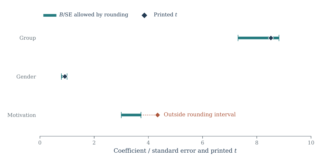
The model is labelled logistic regression, yet the table includes standardized coefficients, \(t\) statistics, and correlation columns, without a defined binary outcome. Renaming it as ordinary linear regression would not resolve all its numerical relationships. Its motivation tolerance and collinearity entry are not reciprocal within their rounding intervals, and a linear-model interpretation creates further disagreement between the coefficients, zero-order correlations, and stated explained variance. These checks constrain interpretation but cannot determine the intended analysis. Accordingly, the present findings make no new adjusted motivational, mediational, or gender claims.
The numerical results are consistent with a higher level of teacher-rated achievement in the design-based learning group during the documented costume-design activities. Both instructional groups engaged with design tasks, while their organization of decision-making and teacher direction differed. The contrast therefore concerns two ways of conducting practical work. It cannot be interpreted as the difference between making artefacts and receiving no practical experience. This distinction matters when connecting the findings to the literature on design thinking, collaborative inquiry, feedback, and learner agency.
Instructional implementation remains consequential to this interpretation. Guidance on formal design-thinking courses addresses course organization and facilitator preparation [34]; professional-development research examines the teacher’s role alongside project characteristics and assessment [35]. Comparisons of design expertise also identify facilitation as a substantive feature of the learning activity [36]. These studies direct attention to how guidance was delivered during costume production, but they cannot identify which instructional component produced the present rating difference.
The narrow ANCOVA coefficient range has a useful educational implication for interpretation: uncertainty about the missing pre–post covariance alone is insufficient to explain away the aggregate separation. By contrast, the assessment-offset analysis identifies a different vulnerability that additional covariance information would not repair. Access to linked scores would sharpen change estimates and permit model diagnostics, but it would not by itself establish independent assessment, equal scoring standards, or the absence of unmeasured allocation differences. Different evidential limitations therefore call for different information.
The findings provide no basis for ranking the five diagnostic domains or attributing the total contrast to communication, reflection, or product creation. Exact domain-level numerical tables and their covariance structure are unavailable. Aggregate scores also embed decisions about item weighting and combination whose measurement assumptions cannot be examined from group means alone [37]. Similarly, the internal consistency coefficients described with the instruments concern relationships among items, rather than agreement between raters or stability across institutions. Treating these properties as interchangeable would give the assessment evidence more support than it possesses. The observed rating difference remains informative when its interpretation is confined to the aggregate outcome actually documented. Formative rubrics may help students understand assessment criteria and use them during learning [38]; this instructional function does not establish agreement between assessors or comparability of scoring across groups.
Transfer is another distinct question. Success in producing and defending a stage costume does not demonstrate performance on an unfamiliar brief, an independently assessed portfolio, or later professional practice. Such outcomes may be educationally desirable, but none is measured in the numerical materials used here. The contribution of the present analysis is to establish how much can be said about the recorded contrast before invoking those broader outcomes. It specifies a robust positive statistical separation alongside unresolved conditions governing its educational and causal meaning.
The calculation also has limits internal to its statistical design. The covariance bounds assume the common-slope linear estimand and unrestricted numerical scores with the stated marginal moments. Unknown score boundaries, ordinal scoring rules, or additional joint constraints could alter the set of feasible student-level records. Conventional confidence intervals additionally rely on sampling assumptions that cannot be checked from the tables. The equal-team calculation does not estimate actual covariance, and the additive displacement cannot represent every form of nonlinear or differential assessment error. These limits are stated with the results because they determine what the calculated ranges mean.
The accompanying machine-readable inputs and calculation scripts preserve the connection between numerical materials, assumptions, and outputs, consistent with the emphasis on provenance and reusable analytical objects in the FAIR principles [39]. Transparent computation allows another analyst to reproduce the arithmetic and inspect its assumptions [40]. It cannot authenticate unobserved individual records or resolve the participant-count disagreement through computation alone.
The research question concerned which conclusions about the instructional achievement contrast remain supported when covariance information is missing and assessment assumptions are made explicit. The answer is that the aggregate contrast is numerically stable, while several broader interpretations remain unidentified. The posttest difference is 0.480 points, and every common-slope adjusted coefficient compatible with the printed group moments lies between 0.458 and 0.502. Two-decimal rounding does not change the direction of that contrast. The difference in mean changes is also positive, but its precision cannot be uniquely determined without the within-person correlations.
Dependence within complete three-person teams increases uncertainty without eliminating the positive lower limit under the illustrative assumptions examined. This result does not establish a causal instructional effect. An unestimated additive assessment difference of approximately 0.283 points would move the lower limit to zero under the largest team design effect, and larger organizational dependencies remain outside that calculation. The evidence therefore supports a positive contrast in the documented ratings whose interpretation depends on allocation and assessment conditions that the aggregate numbers cannot verify.
The methodological contribution is the explicit separation of coefficient identification, conditional sampling uncertainty, and systematic displacement. These quantities respond differently to the same incomplete report. Missing covariance leaves a narrow range of adjusted group coefficients because the pretest group means are close; it leaves a much wider range of uncertainty for change. Neither result resolves incompatible gender and motivation entries, establishes equivalent gender outcomes, or identifies why students obtained different ratings. A defensible educational conclusion is consequently limited to the observed instructional comparison and the clearly stated models under which its statistical properties were calculated.
The practical consequence is that information must match the claim being evaluated. Paired scores would determine change uncertainty; team identifiers would support dependence estimation; independent ratings would address assessment comparability. None of these additions can be replaced by stronger wording around existing probability values, and the numerical bounds should remain attached to the assumptions under which they were derived and interpreted.
The numerical inputs, their corresponding table and page locations, calculation scripts, independently generated figure panels, and computational outputs accompany this manuscript. These files contain aggregate statistics and no individual student records. The accompanying Python programs reproduce the numerical tables and figures without requiring network access.
The author declares no conflicts of interest.
The author received no specific funding for this research.
Artificial intelligence tools were used to assist with programming and numerical verification. The author takes full responsibility for the content of the manuscript.